Mastering Hexapawn AlphaZero-style
Hexapawn is a two-player, full-information, deterministic game (black always has a winning strategy). It was designed by Martin Gardner and published in an article where he described how to build a game-learning machine using 24 matchboxes. I got interested in this while reading the book called Neural Networks for Chess. Actually, the book also has its own implementation of HexapawnZero. I decided to implement it myself so that I understand it well, even though many parts of my implementation are heavily inspired by that of the book.
When we try to devise algorithms to play a two-player game, we end up working with a game tree where the nodes of the tree signify board position or one of many possible states of the game and the edges in the tree refer to a valid move to play or an action that can be taken from the state.
When we want to select one move from the set of all possible valid moves, we need to somehow evaluate the states we end up with upon playing the moves. Hexapawn is a very simple game where a match only lasts for five or six moves at most. For simple games like Hexapawn or Tic-Tac-Toe, it’s very easy to build up the whole tree from the current state considering all possible attainable states. Thus we can choose our move in such a way that the terminal node in the tree is in our favour. But for games like Chess or Go, it’s not at all feasible to build up the whole tree. For example, a typical chess game consists of 40 moves and in each move there are on average 35 valid actions to choose from (i.e., the full tree will have breadth and depth as 35 and 40 respectively, containing \(35^{40}\) possible sequences of moves). For the game of Go it’s even worse (~ \(250^{150}\) possible sequences of moves, more than the number of atoms in the universe!). Games like these are known to have high-branching factors. So we have to stop at some point and estimate how the final positions would look from the leaf nodes in the tree.
There are many ways to evaluate a board position. For example, in Chess, a very crude and simple way of doing it is to count the number of pieces one player has compared to the opponent. A little modification of this can be done by not just simply counting the pieces but calculating a weighted sum of the pieces (Queens for 8 points, Knights for 3 points, etc.). As we can imagine, there can be countless number of handcrafted evaluation functions that one can think of. Also, different games need different evaluation functions. Simple evaluation functions like the ones mentioned earlier are not very robust (think of a situation where you are up a rook, a bishop and a knight but you are playing against Tal!)
The way Monte-Carlo Tree Search (MCTS) evaluates a leaf node is very simple. It plays a number of matches from the position by making a random sequence of moves for both the players and then uses the winning ratio to calculate the value of the node. So, it’s kind of like sampling from all possible games that can be played from that state and then estimating the true value of it by the score obtained from matches present in the sample. Here are the four steps of MCTS for building up and traversing the tree.
- Selection (starting from the root node select successive child nodes until a leaf node is reached)
- Expansion (expand the leaf node by adding one or more nodes with states attainable from it by playing valid moves)
- Simulation (play a series of games choosing random moves for both the players)
- Backpropagation (update the node statistics, namely the visit counts and the expected values, using the simulation result)
The MCTS in AlphaZero is a modified version of the original MCTS algorithm. It replaces the simulation step with a Neural Network evaluation (taking out the ‘Monte-Carlo’ part from MCTS if you think about it 😅). It also incorporates policy in the selection part of MCTS.
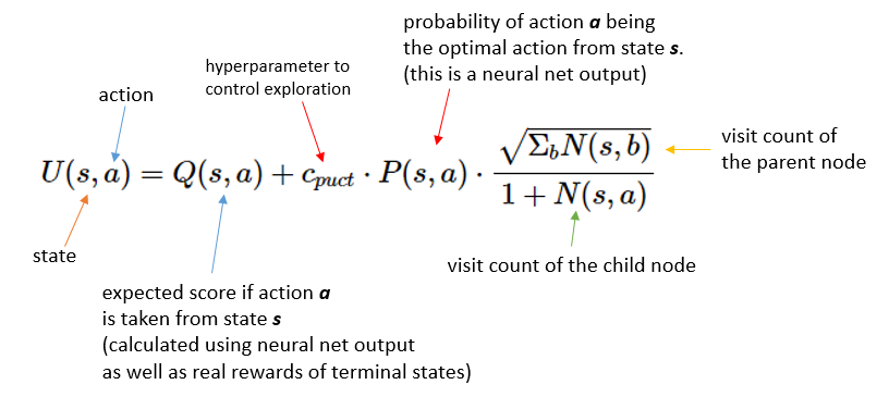
Each node has a few statistics stored with them. One of them is the Q value, which is the expected score you get by playing from the state represented by the node. It lies between -1 and 1 (1 if the player wins, -1 if they lose). To select a child node to traverse through, we calculate the UCT (Upper Confidence bounds applied to Trees) value of all the child nodes and then select the one with the maximum UCT value. The UCT value is calculated using the below formula:
The Neural Net
The neural network that we are going to be using (HexapawnNet) is very simple. The input is a 21-dimensional binary vector. The first 9 elements signify the white piece positions, the next 9 elements are for black piece positions and the remaining 3 elements are set to 1 if it’s white’s turn or 0 if it’s black’s turn.
>>> state = np.array([[-1, -1, 0], [0, 1, -1], [1, 0, 1]])

>>> draw_board(state)

    +-----+-----+-----+
 0  |  B  |  B  |     |
    +-----+-----+-----+
 1  |     |  W  |  B  |
    +-----+-----+-----+
 2  |  W  |     |  W  |
    +-----+-----+-----+
       0     1     2

>>> print("Input:", get_input_from_state(state, player=1))

Input: [0 0 0 0 1 0 1 0 1 1 1 0 0 0 1 0 0 0 1 1 1]
HexapawnNet consists of four fully connected layers with 128 neurons each and ReLU activation function. The fourth layer is then connected to a policy head and a value head. The policy head outputs a probability vector of length 28 (since there are 28 possible moves: 6 forward moves, 8 capture moves for both black and white, as stored in a dictionary here). The value head goes through the tanh activation function which produces a value in between -1 and 1. The neural net is trained to minimize the sum of the mean-squared error (of the value output) and the cross-entropy loss (of the policy output).
During the MCTS iterations when we are at an unvisited leaf node which is not a terminal node (i.e., the game has not ended yet), we update the node policy with the masked neural net policy and the node value with the neural net value output. Masking is necessary because the actual policy output from HexapawnNet can allocate non-zero probabilities to illegal moves.
>>> state = np.array([[0, -1, 0], [0, -1, 0], [1, 0, 1]])
>>> draw_board(state)

    +-----+-----+-----+
 0  |     |  B  |     |
    +-----+-----+-----+
 1  |     |  B  |     |
    +-----+-----+-----+
 2  |  W  |     |  W  |
    +-----+-----+-----+
       0     1     2

>>> inp = get_input_from_state(state, player=0)
>>> hnet = HexapawnNet()
>>> p, v = hnet.predict(inp)
>>> print(mask_illegal_moves(state, torch.exp(p), 1))

[0.24404633 0.         0.24610272 0.         0.         0.
 0.         0.         0.         0.         0.         0.
 0.25840706 0.         0.         0.25144392 0.         0.
 0.         0.         0.         0.         0.         0.
 0.         0.         0.         0.        ]


>>> print(v)

tensor([0.1034])
Example Generation
As we can see from the above code snippet, the randomly initialized neural network is returning a policy where the total probability is distributed more or less evenly among all the legal moves. What we instead want is to have higher probabilities for good moves. To train the neural net, we need examples games to train it on. AlphaZero’s predecessor AlphaGo followed a supervised learning method where it was trained on millions of games played by professional Go players. On the other hand, AlphaZero is trained on games which were generated by itself. To do so we need data points of this form: [state, target-policy, target-value], i.e., when the input to HexapawnNet is state, we want the output policy and value to be as close as possible to the target-policy and the target-value. Here’s how we generate them using the neural net itself.
We play a number of games by doing a bunch of MCTS iterations from the starting position. Each of the games we play provides us with a few examples. We use the neural net to calculate the policy and the value which then are used to calculate the UCT value required to build up and traverse the tree. After building up the tree, we have an improved policy from the node statistics of the tree (namely, the relative visit counts). We update the dataset by appending it with [current state, improved policy, None]. The value is set to None until we have the actual reward after the end of the game. Next we sample a move using the improved policy as the move probability distribution and repeat the process from the state obtained after playing the sampled move from the previous state.
Here’s how the training data might look like after one game:
    +-----+-----+-----+
 0  |  B  |  B  |  B  |   input: [0, 0, 0, 0, 0, 0, 1, 1, 1, -1, -1, -1, 0, 0, 0, 0, 0, 0, 1, 1, 1]
    +-----+-----+-----+
 1  |     |     |     |   target-policy: [0.33333333, 0.33333333, 0.33333333, 0.0, 0.0, 0.0, ... ]
    +-----+-----+-----+
 2  |  W  |  W  |  W  |   target-value: -1  (since White lost)
    +-----+-----+-----+
       0     1     2

player: white


    +-----+-----+-----+
 0  |  B  |  B  |  B  |   input: [0, 0, 0, 1, 0, 0, 0, 1, 1, -1, -1, -1, 0, 0, 0, 0, 0, 0, 0, 0, 0]
    +-----+-----+-----+
 1  |  W  |     |     |   target-policy: [0.0, 0.0, 0.0, 0.0, 0.0, 0.0, 0.0, 0.33333333, 0.22222222, ... ]
    +-----+-----+-----+
 2  |     |  W  |  W  |   target-value: 1  (since Black won)
    +-----+-----+-----+
       0     1     2

player: black


    +-----+-----+-----+
 0  |  B  |     |  B  |    input: [0, 0, 0, 0, 0, 0, 0, 1, 1, -1, 0, -1, -1, 0, 0, 0, 0, 0, 1, 1, 1]
    +-----+-----+-----+
 1  |  B  |     |     |    target-policy: [0.0, 0.55555556, 0.22222222, 0.0, 0.0, 0.0, 0.0, 0.0, 0.0, ... ]
    +-----+-----+-----+
 2  |     |  W  |  W  |    target-value: -1
    +-----+-----+-----+
       0     1     2

player: white


    +-----+-----+-----+
 0  |  B  |     |  B  |   input: [0, 0, 0, 0, 1, 0, 0, 0, 1, -1, 0, -1, -1, 0, 0, 0, 0, 0, 0, 0, 0]
    +-----+-----+-----+
 1  |  B  |  W  |     |   target-policy: [0.0, 0.0, 0.0, 0.0, 0.0, 0.0, 0.0, 0.0, 0.11111111, 0.66666667, 0.0, ... ]
    +-----+-----+-----+
 2  |     |     |  W  |   target-value: 1
    +-----+-----+-----+
       0     1     2

player: black
Policy Iteration with Self-Play
Now that we can generate examples to train our HexapawnNet on, we will initialize it with random weights, generate a bunch of examples using the Neural Net doing MCTS, and then train the neural net on these examples. Now we have an improved model that we will pit against its older version. If the winning ratio of the trained network exceeds some pre-specified threshold, we swap the old net with the trained one and continue this process. Otherwise, we augment the training data with a new set of examples. Since Hexapawn is a pretty simple game, it takes us only a few iterations for the neural net to figure out the winning strategy for black. As we go through more and more iterations, we expect HexapawnNet to win most if not all the games it plays as black. Also, after a bunch of iterations it starts to lose all the games it plays as white because by that time its opponent (which is just its own older version) has also learned how to win as black! This is exactly what we see when we go through ~5 episodes of self-play.
$ python self_play.py

Iteration: 1
As black: 10 out of 10
As white: 4 out of 10
Total Wins:  14
frac_win:  0.7
------------------------------
Iteration: 2
As black: 10 out of 10
As white: 1 out of 10
Total Wins:  11
frac_win:  0.55
------------------------------
Iteration: 3
As black: 10 out of 10
As white: 0 out of 10
Total Wins:  10
frac_win:  0.5
------------------------------
Iteration: 4
As black: 10 out of 10
As white: 0 out of 10
Total Wins:  10
frac_win:  0.5
------------------------------
Iteration: 5
As black: 10 out of 10
As white: 0 out of 10
Total Wins:  10
frac_win:  0.5
------------------------------
As black: 25 out of 25
As white: 15 out of 25
Total Wins:  40
Final Score with untrained NN: 0.8
Acknowledgments
Neural Networks for Chess is the book that first got me interested in this project. My implementation is broadly based on the one in the book. Whenever I read the original paper, I felt that I understood everything and then when I went on to implement them myself, I realized that I did not fully understand many things. I resorted to A Simple Alpha(Go) Zero Tutorial during those times.