Mixture Density Networks
Probabilistic Interpretation
When we have a dataset of the form \(\{(Y_1, x_1), (Y_2, x_2), ... (Y_n, x_n)\}\) (here \(Y\) is a scalar and \(x\) can be either a scalar or vector-valued) and we want to fit a regression model with it, we assume a functional form of our dataset: \(Y = w \cdot x + \epsilon\) where \(\epsilon\) is the error part in our prediction and \(w\) is the unknown weights. We formulate a loss function of the form \(\sum_i (Y_i - w \cdot x_i)^2\) and find the value of \(w\) which minimizes the loss.
Now, wouldn’t it be nice to not just predict the value of \(Y\) given \(x\), but the distribution of \(Y \mid x\)? Turns out that there’s also a probabilistic interpretation of the regression model.
\[Y_i = w \cdot x_i + \epsilon_i\]In the above formulation, we can assume \(\epsilon_i\) -s to be independent and identically distributed (IID) random variables originating from a Gaussian distribution with mean \(0\) and some variance \(\sigma^2\), which means the distribution of \(Y_i\) conditioned on \(x\) is another Gaussian distribution with mean \(w \cdot x_i\) and variance \(\sigma^2\). Note that values of all \((Y_i, x_i)\) pairs are known to us. So, to estimate the coefficient’s value, we can use Maximum Likelihood Estimation (or MLE, where we write down the joint pdf of \(\{Y_1, Y_2, ..., Y_n\}\) and find the value of \(w\) which maximizes it). The MLE of \(w\) turns out to be the same as what we get when we minimize the Mean Square Error loss. It should be mentioned here that, if we consider \(w\) to be another random variable with its density function then instead of MLE, we would be doing a Maximum a posteriori estimation (MAPE), and depending on different distributional assumptions of \(w\) we get all sorts of nice interpretation, e.g., assumption of \(w\) to be following a Gaussian or Laplace distribution gives rise to L2 and L1 regularization respectively.
In the regression example, we made an assumption about the Gaussian distribution of the error parts which made the distributional form of \(Y \mid x\) known to us. What if we are using a neural network? Neural Networks are great function approximators. So, instead of predicting the y-value, it can be used to output a distribution or rather the parameters of a distribution. That’s great but what if we do not know about or make any assumption on the distributional form of \(Y \mid x\)? This is where the Gaussian mixture model comes into play. Turns out a Gaussian mixture model is a universal approximator of densities; or in other words, any smooth density function can be approximated as a weighted sum of a suitable number of Gaussian density functions with appropriate means and variances1.
The Forward Problem
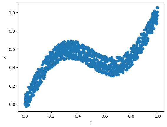
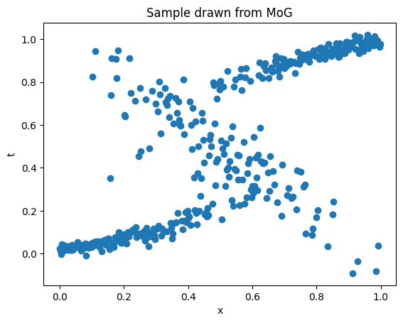
In his 1998 paper on Mixture Density Networks2, Bishop considered a simple example to showcase the usefulness of Mixture Density Networks (MDN) in problems where a simple Network would fail. We will use the below equation to generate the training data.
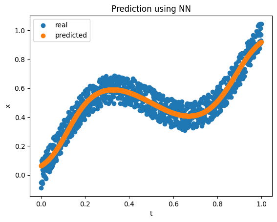
\[x = t + 0.3 \sin(2 \pi t) + \epsilon\]where \(\epsilon \sim U(-0.1, 0.1)\). We sample 1000 points using the above equation and choose \(t\) at equal intervals in the \((0.0, 1.0)\) interval. If we consider the forward problem or mapping \(x\) from \(t\), a simple network with 1 input, 5 hidden inputs with tanh activation, and 1 output works pretty well.
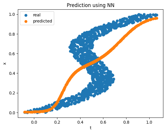
The Inverse Problem
What if we consider the inverse problem, where, given the value of \(x\) we have to estimate \(t\)? Note that we have more than one value in some regions for a given value of \(x\). A similar neural net does not fare well in this case, especially in the regions where there are multiple \(t\) values for a single \(x\) value.

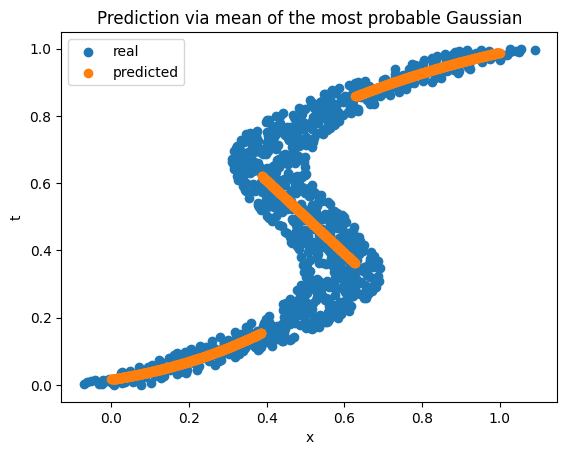
MDN solves the inverse problem very nicely. The idea is to predict the distribution of \(t\) conditioned on \(x\). This distribution is expressed as a mixture of Gaussian distributions, i.e., \(f(t \mid x) = \sum_{i=1}^m \pi_i \phi_i(t \mid x)\), where \(\sum_{i=1}^m \pi_i = 1\) with each \(\pi_i \ge 0\) and \(\phi_i\) is the pdf of a Gaussian distribution. If there are \(m\) number of independently distributed Gaussians then the neural net output would be a \(3m\) dimensional vector (\(m\) mixture coefficients, \(m\) means, and \(m\) variances). The number of Gaussians to use may not be known beforehand but the idea is that even if we end up overestimating the number of Gaussians needed, the predicted mixture coefficients for the unimportant Gaussians will be close to \(0\) making them not impactful to the final result. Also, to make sure that the predicted mixture coefficients sum up to be 0 and the variance estimators stay positive, we need to pass the corresponding output to a softmax activation or exponentiate them before using them to construct the loss function (see here for the actual implementation). Since we have a probability distribution as the output, we will use the negative log-likelihood instead of MSE as the loss function for minimization.
Okay, but how do we predict a single value if we have a mixture of Gaussians as the output? There are several ways to do this. One way is to just use the mean of the Gaussian corresponding to the maximum mixture coefficient (i.e., the center of the most probable kernel). This gives a discontinuous functional mapping from \(x\) to \(t\).
Alternatively, we also can sample from the output distribution itself. For this, we first determine which Gaussian to choose the final sample from by doing a random sampling from the set of Gaussians using the mixture coefficients as the probability and then draw a sample point from the chosen Gaussian. How do we make sure doing these two steps is equivalent to actually sampling from the MoG? For this, note that, if \(X\) is the random variable obtained from following the above two steps, then the cumulative distribution function (CDF) of \(X\) can be written as,
\[\begin{align*} P(X \le x) &= \sum_i P(X \le x \mid \text{x coming from i-th Gaussian}) \cdot P(\text{choosing i-th Gaussian}) \\ & = \sum_i \Phi_i(x) \cdot \pi_i \end{align*}\]where \(\Phi_i(x)\) is the CDF of i-th Gaussian and \(\pi_i\) is the i-th mixture coefficient. Now we just differentiate the CDF w.r.t. \(x\) to get the density function of \(X\), which turns out to be the same as the MoG!
Code to reproduce the results can be found here.
References
-
I. Goodfellow, Y. Bengio, and A. Courville, Deep Learning, MIT Press, 2016. ↩
-
Christopher M. Bishop, Mixture Density Networks ↩