Watermarking LLM Output
Large Language Models (LLMs) can be thought of as a function that takes as an input a sequence of tokens and spits out as output the probability distribution of the next token. The main idea behind LLM watermarking is to change the generated text in such a way so that the quality of the text remains the same (non-distortionary change, i.e., no noticeable change from the perspective of a human reader) but it becomes detectable if you have access to the things that were used to watermark it in the first place. Identifying machine-generated text is a crucial challenge with immense implications for detecting academic plagiarism or preventing the proliferation of machine-generated content and social media bots on the internet.
So, what do we expect a good watermarking scheme to have? Well, first of all, it would be nice to have it not requiring white-box access to or modifying in any way the language model itself. Secondly, we want the results post-watermarking to be not much worse than the original model output (it’s ok to compromise a little bit on quality). Additionally, we would like the scheme not to mess up low-entropy scenarios. For example,
the token Barack is almost deterministically followed by Obama in most cases, so we do not want our watermarking scheme to accidentally disallow Obama. Lastly, we would like to have a robust statistical measure of confidence in detection time.
There are various approaches to do this but this post will essentially summarise two watermarking schemes. I may update this later to include more schemes.
The Red-Green Split
The first watermarking scheme as described by Kirchenbauer et al1 is the “hard” red-green list split. The idea is to split the vocabulary into two sets - a set of green tokens and a set of red tokens, where we are only allowed to sample the next token from the green set. This splitting is supposed to be done randomly but it’s also a function of the last (or last few) token(s), which means that the random seed to be used for splitting the vocabulary set into two sets is going to be an output of a hash function which uses the last token(s) as input. Now, for texts generated by a non-watermarked LLM, we should see a more or less equal number of red tokens and green tokens, but for a watermarked output, we expect to see a higher number of green set tokens. (note that during detection time, when we are determining the count of green tokens, we have full information about the green and red lists at each step). More formally, if we have a sequence of tokens of length \(T\) and the proportion of green tokens in the vocabulary is \(\gamma\), then the number of green tokens in the text, \(\mid s\mid _g\) will follow a \(\text{Binomial}(T, \gamma)\) distribution. If we use a Gaussian approximation then the \(z\)-statistic will be \(\frac{\mid s\mid _g - \gamma T}{\sqrt{T \gamma (1-\gamma)}}\) which can be used to calculate p-value or to come up with a threshold above which we accept the text to be watermarked. This is a “hard” split in the sense that, once we construct the red and green sets, we completely forbid the red tokens to appear in the sample. This can be detrimental to the quality of the text, especially in the low-entropy sequences (if you accidentally end up having many high-probability tokens in the red list).
This leads us to the “soft” split. In this case, we still divide the vocabulary into two sets of red and green tokens, but now, we try to artificially bump up the probabilities of the green tokens hoping that this will lead to them appearing in the sample more frequently than their red counterparts. This is done by adding a small scalar \(\delta\) to the logits associated with green tokens before taking softmax. If \(V\) is the vocabulary, \(G\) and \(R\) denotes the green and red set of tokens and \(l = \{ l_1, l_2, ..., l_{\mid V\mid } \}\) is the logits, then probability \(\hat p_k\) of a token at index \(k\) becomes the following.
\[\hat p_k = \begin{cases} \frac{\exp(l_k + \delta)} {\sum_{i \in R} \exp(l_i) + \sum_{i \in G} \exp(l_i + \delta)}, & k \in G & \\ \frac{\exp(l_k)} {\sum_{i \in R} \exp(l_i) + \sum_{i \in G} \exp(l_i + \delta)}, &k \in R \end{cases}\]Note that this does not have a negative impact on the quality of the text at low entropy scenarios since adding a small amount to the logits will not have that much of an impact when a highly likely token has a very large logit. This is the soft split in the sense that, the red tokens can still appear in the sample albeit with a very small likelihood. The test statistic and p-value calculation and other things remain identical.
SynthID
The core concept of the recent work done by Dathathri et al.2 at Deepmind involves employing one or more pseudo-random functions to score each generated token during inference and selecting the tokens with the highest scores. When we are given a sequence of tokens to determine if it’s generated by a watermarked LLM, we will calculate the mean score of the tokens (using those same functions mentioned earlier) and if it’s larger than some threshold we will say that it’s watermarked. We will talk about the function in a bit, but for now, let’s assume that we have such a function that takes as an input a sequence of tokens and spits out either 0 or 1. In the paper, they use the tournament sampling technique which is explained next.
Let’s say, the input to the LLM is “My favorite tropical fruit is”. Let’s also fix the number of rounds in the tournament to 3. This means, we first sample \(8 (= 2^3)\) tokens (one token can appear multiple times) from the LLM distribution and split them into pairs of competing tokens. We will also have 3 random functions (referred to as \(g_1, g_2\) and \(g_3\)). The highest scoring tokens from one layer (\(g_i\) is used for scoring in layer \(i\)) are moved to the next layer (in case of a tie, we choose one token randomly). The below diagram from the paper should be self-explanatory.
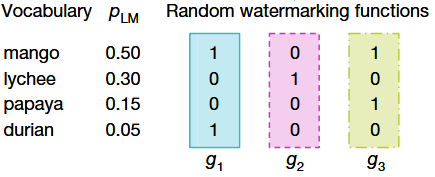
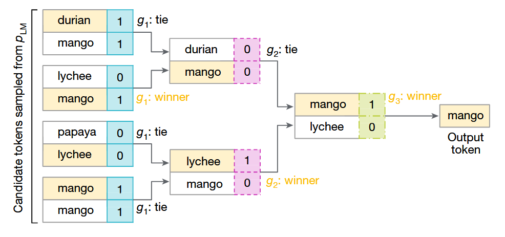
Fig.1 - Tournament Sampling in SynthID.
So, the basic idea is that, given a sequence of watermarked tokens, if you calculate the mean token scores \(\frac{1}{mT}\sum_{l=1}^m \sum_{t=1}^T g_l(x_t, r_t)\), where \(m\) is the number of layers, \(T\) is number of tokens in the sequence, the watermarked text is expected to score higher than a non-watermarked text (the threshold can be chosen empirically).
Ok, but what do we use as the g-function? And why does it have to be random? Can it be deterministic? Well, we want it to be random because if they are not, then we may accidentally end up being biased toward some specific set of tokens (which can deteriorate the quality of the generated text).
In the paper, they used the \(g\)-function of a layer as a function that takes as input a number of previous tokens and a random seed. The distribution of the output of this function can be \(\text{Bernoulli}(0.5)\) (like in our previous example) or \(\text{Uniform}[0, 1]\). Once we fix the distribution, we will use the Probability Integral Transform (PIT) to sample from it. PIT states that for a random variable \(X\), irrespective of what distribution it has, the Cumulative Density Function (CDF) \(F_X\) will always have a Uniform[0, 1] distribution. This is great because now to sample from any distribution we just need to know the CDF of that distribution and we need to know how to sample from Uniform[0,1]. For example, let’s say \(Y\) is a random variable with CDF \(F_Y\). To sample from the distribution of \(Y\), we sample a Uniform[0,1] distribution \(u\) and then solve for \(y\) in the equation \(F_Y(y) = u\).
At first, we fix the distribution that we want the g function to follow to, say, \(F_g\). Then we draw a sample from \(\text{Uniform}[0, 1]\) distribution conditioned on a number of previous tokens. To do this, at first, we use a hash function (\(f_r\)) which takes previous \(H\) (referred to as ‘context window’) tokens \((x_{t-H}, ..., x_{t-1})\), the layer number \(l\) and a random key \(k\). Randomizing the key will randomize the hash functions. Let’s call the output of this function, the random seed, \(r\). Next, another similar hash function (\(h\)) is chosen which takes as input a token \(x\), the layer number \(l\) and the random seed \(r\) and the output \(h(x, l, r)\) is an \(n_{sec}\)-bit integer. We divide this output by \(2^{n_{sec}}\) so that it lies in [0, 1]. Now we use PIT and evaluate the generalized inverse of \(F_g\) at this point. So finally the g-value for context \(x_{<t} = (x_{t-H}, ..., x_{t-1})\), layer \(l\), token \(x\) becomes
\[g_l(x, r) = F_g^{-1} \left( \frac{h(x, l, f_r(x_{<t}, l))}{2^{n_{sec}}} \right)\]Limitations
Despite their robust mathematical foundation, the discussed watermarking schemes are susceptible to attacks such as paraphrasing (using human attacker or another LLM), the “Emoji Attack” (where the LLM is asked to inject emojis in between words and later these emojis are discarded and only the text is used), etc. Even though they are empirically proven to be somewhat robust to these types of attacks to some extent, they do not offer a complete solution to machine-generated text detection which leads us to the question of whether it is possible to design a watermarking scheme that operates at a semantic level.
References
-
Kirchenbauer, J., Geiping, J., Wen, Y. et al. A Watermark for Large Language Models. ↩
-
Dathathri, S., See, A., Ghaisas, S. et al. Scalable watermarking for identifying large language model outputs. Nature 634, 818–823 (2024). https://doi.org/10.1038/s41586-024-08025-4 ↩